Lecture 5 - Recurrent Neural Networks

Language Models#

It was always believed that you couldn’t possibly train a model which has billions of parameters. As it turns out, we now have models that have millions of parameters in the form of language models.

The myth of overfitting#

It is also observed that when we train a very deep neural network with billions of parameters, overfitting is kind of a myth. There appears a point at which it seems like the model is overfitting, but, as you train it more, the loss converges. It is a very common practice to heavily overfit language models (owing to their large number of parameters).

Dropout#

Choosing a ratio. This ratio is the percentage of the neurons that will be switched off during training of the model.

This ensures that dependency of the model is not exactly on a certain few neurons, instead it is spread across all the neurons of the model.

Parameter initialization#

When we initialize parameters in a model's matrix of weights. We almost always initialize it to random numbers instead of initializing it to zeros. This is done because we observe that a lot of the functions are symmetric about to the axis meeting points. These points are called saddle points. We try our best to avoid them.

Optimizers#

For usual networks, SGD works just fine. If we want to work with deeper neural networks, then we need to also look into more sophisticated optimizers like

• Adam --> a good place to start
• Adagrad
• RMSprop
• AdamW
• NAdamW --> Better for Word Vectors Hyperparameter tuning is another thing we need to get better at. The only way we could get better with this is by training more and more models. A good place to start is $10^{-3}$.

Language Models#

They are built with the main purpose of guessing the next word that comes in context. The guessing is done using probabilities.

N-gram language model#

An n-gram language model is a model that clubs together $n$ number of consecutive words together. The model maps probabilities for each of these chunks. So, for instance, we see a chunk of words, we train the model to give probabilities of which chunk might appear next.

To say the least, this is a very prude and primitive model. Without a larger context, it is very hard to guess what the next word is.

• Sparsity Problem: We could say, we could take larger chunks of words and make probability distributions for smaller chunks or maybe just a singular word. This could work better, but what if the larger chunk of words never occurred in the training corpus of text. One thing we could do is reduce the size of the chunk, this is called backoff. In most cases, we cannot have n more than 5.
• The Storage Problem: We would need to store a crazy amount of data to remember the probabilities of every single combo of words.
  It is easy to built though.

We tend to use this more for next word prediction on out phones, not for text generation.

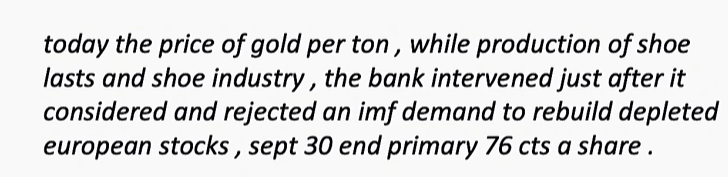
Here is an example of a model that was trained on 2 million words on a trigram model.

Neural Language Model#

The idea is pretty simple, we have a context window. We grab all words in this context window and then whichever word are in the vocabulary are converted to one hot encodings, then the target word is also converted to its respective one hot encoding. Later this is passed through a neural network and the final label is the target word.

This way we train the model to learn relations between words words.

Neural Language models are not exactly limited to just next word prediction. They can classify text as well, maybe semantically, or based off the language it was written in, and so on.

The issue with this is that the context window can never be long enough.

Recurrent Neural Networks (RNNs)#

Vanilla RNNs#

What sets apart a Vanilla RNN from an ANN?#

A Vanilla RNN also has a feedback loop along with the traditional Weights, biases, and activation functions.

Training a Vanilla RNN for Named-Entity Recognition (NER)#

We obviously need a huge corpus of data. We first split this into batches. Each batch can be imagined as a sentence for simplicity.

Inside each of the sentences, we spilt them into words and if the word is a Named-entity, we can label it positive, else negative. The simplest way to do this, is by making a vector of zeroes and ones. The vector should contain as many cells as the number of words in the batch. Each cell corresponds to a word in the batch. One if it is a named entity, Zero if it is not a named entity.

Let us assume we have a bunch of batches:

Dhaval loves Baby Yoda -> {1, 0, 1, 1}
Bob told Ahmed that pizza is delivered -> {1, 0, 1, 0, 0, 0, 0}
Ironman punched Hulk's face -> {1, 0, 0, 1, 1}

Let us now take the first batch, we have randomly assigned the weights and biases to the RNN.

This RNN here has one neuron in its input layer, one neuron in its hidden layer, one neuron in its output layer.

In an RNN, we observe a feedback loop between the terminals of the hidden layer. This is the main difference between an RNN and an ANN. At every Run of the RNN, we grab the output of the hidden layer. During the next Run of the RNN, we make sure we add in the weighted sum of the previously grabbed output to the value we were about to pass through the activation function. After adding these, we pass them through the activation function. This is done until the sequence comes to an end.

Here, when we say batch, we are referring to the same sequence. Let us take a look at a representation of a very simple RNN, which we could use to build a very simple NER model.

NOTE: Keep in mind that OHV stands for One-hot vector.

Now this is a bit confusing to look at, so let me break this down.

What we have done here is called Unfolding an RNN. Keep in mind that this is still the same neural network we have seen before, but we can now look at it more like a timeline. Each word initiates a Run of the RNN. After each run we pass the value to the next run's weighted sum.

At each run, we calculate the losses by comparing the loss of the predictions of that run to the label we saw earlier. We accumulate all these losses and backpropagate once the entire batch is completed. This backpropagation is done on the total loss, not individual losses.

Now, we do the same for each batch, and keep backpropagating once per batch. We often run multiple epochs until loss converges.

The backpropagating method i mentioned above is called Truncated Backpropagation. We could also just run backpropagation every run and it would still work out.

The issue with Vanilla RNNs#

We mainly observe two issues with Vanilla RNNs:
Take a closer look at the weight with which we multiply the value when we transfer it between any two consecutive runs of a sequence. Here is where the issue lies.

• Exploding Gradient If this number is greater than unity, the value we get on the first run is very amplified as we reach the last run. Let us assume the weight is $1.8$. By the time it gets to the fourth run, the first run's value is amplified by a weight of $1.8^{4} = 10.496$ in the gradient. What this essentially means is, the leaps taken by the optimizer to reduce loss is extremely large. Meaning, we would be jumping around space, without really finding the minima.
• Vanishing Gradient If the number is lesser than unity, the value we get on the first run is reduced to a great extent. Meaning the overall leaps would be way too small to reach the minima. We would just end up not moving too far from our initial point even after training the model for a significant amount of time.