Linear Regression · Vrishank Aryan S

Linear and Logistic regression are the backbone of almost all older ML models. Any model with its decision boundary of the form:

Y=W^TX+B

(where (Y) is the label, (X) is the feature matrix, (W) is the weight matrix, and (B) is the bias, a scalar value) is called a Linear Model.

Let me quickly walk you through the key differences between Linear Regression and Logistic Regression.

Linear Regression	Logistic Regression
Used to predict a value (label) when given corresponding features.	Used to classify between two clusters given features. It gives a boolean output.
Error is measured using Mean Square Error (MSE).	Error is measured using Binary Cross Entropy (maximizing negative log likelihood).

Linear Regression#

Here's how a computer solves a Linear Regression problem:#

You begin with a table of features (X) and labels (Y). Suppose there are M training examples and N-1 features.

$X_{1}$	$X_2$	$X_3$	$X_4$	$Y$
2	4	6	8	114
4	6	8	10	168
9	11	13	15	343

Here, (M = 3) and (N-1 = 4.

To include a bias, add an extra column filled with 1s to your feature matrix:

$X_0$	$X_1$	$X_2$	$X_3$	$X_4$	$Y$
1	2	4	6	8	114
1	4	6	8	10	168
1	9	11	13	15	343

Then initialize a weight vector $W$ , often with zeros:

$Bias/W_0$	$W_1$	$W_2$	$W_3$	$W_4$
0	0	0	0	0

Feature and Label Matrices:#

Features (X):

$X_1$	$X_2$	$X_3$	$X_4$
2	4	6	8
4	6	8	10
9	11	13	15

Labels (Y):

114

168

343

Error Function: Mean Square Error#

We use the Mean Square Error (MSE) as our loss function and Gradient Descent to optimize:

\text{MSE}=\frac{1}{m}\sum_{i=1}^{m}(Y_i-\hat{Y_i})^2

Where:

$Y_i$ is the actual label,
$\hat{Y_i}=h_\theta(X_i)$ is the predicted label,
$h_\theta(X_i)=X_i\cdot W$

Optimizer: Gradient Descent#

Update rule:

\theta_j:=\theta_j-\alpha\cdot\frac{\partial J(\theta)}{\partial\theta_j}

For MSE, this becomes:

\theta_j:=\theta_j-\alpha\cdot\sum_{i=1}^{m}(h_\theta(X_i)-Y_i)\cdot X_{ij}

You repeat this for every ( $\theta_j$ ) in the weight matrix until convergence.

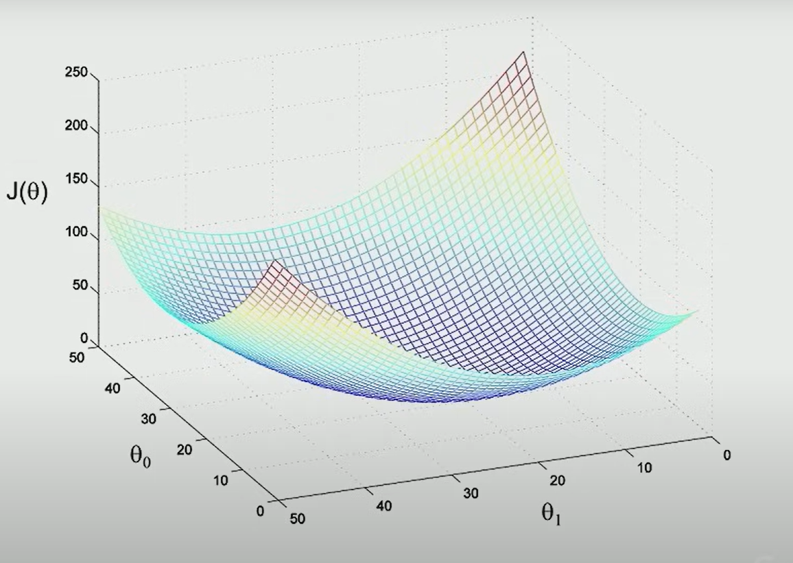
Visualizing the Loss Surface#

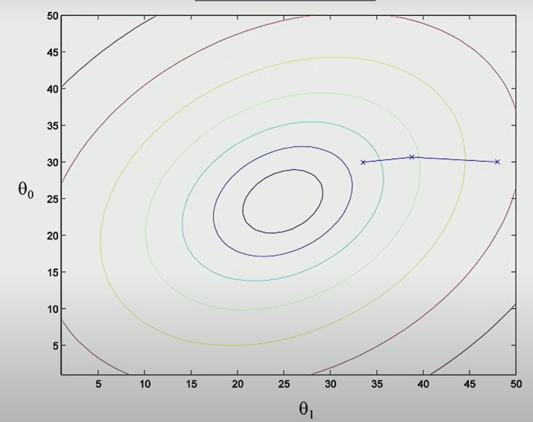
In the case of two weights $\theta_1$ , $\theta_2$ , the loss surface $J(\theta)$ is a convex bowl-shaped curve with a single global minimum. This is why gradient descent works so effectively.

Contour Plot:

Final Weights (after optimization)#

$Bias/W_0$	$W_1$	$W_2$	$W_3$	$W_4$
10	5	7	2	8

Verifying Predictions#

First training example:

$X_0$	$X_1$	$X_2$	$X_3$	$X_4$
1	2	4	6	8

Predicted:

Y=X\cdot W^T=[1\ 2\ 4\ 6\ 8]\cdot[10\ 5\ 7\ 2\ 8]^T=114

Second training example:

$X_0$	$X_1$	$X_2$	$X_3$	$X_4$
1	4	6	8	10