Logistic Regression · Vrishank Aryan S

Logistic Regression in simple terms is an adaptation of Linear Regression to classify between clusters of data-points with a line (or a curve, i will speak more about how to get a curve later).
The key differences made here are:
- $Y_i$ $Y_{i}$ , $\forall$ $\forall$ i $\in$ $\in$ (1, M) = {0, 1}
  - Meaning for a $Y_i$ , the label, will always be either 0 or 1.
- We still maintain the same hypothesis, $h_\theta$ $h_{θ}$ , with a tiny change. After calculation of $h_\theta$ $h_{θ}$ , we pass it though the Sigmoid function.
  $Sigmoid(z) = \frac{1}{1+e^-z}$
  - Why sigmoid though?
    - Here is the graph of sigmoid:
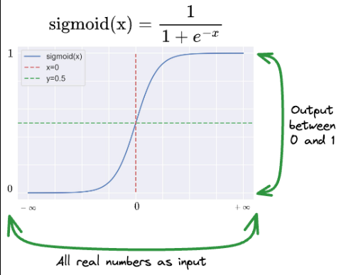
    - As we can see, it has all real numbers as domain, but its range is between 0 and 1.
    - This is valuable because, once we calculate $h_\theta$ , we pass it through the Sigmoid, This gives us the same $h_\theta$ in the range 0 to 1. Meaning, we can classify it as 0 if below, 0.5 and as 1 is above 0.5.
- We use Negative log-likelihood for our error measurement.
  - Likelihood gives us the same output, but we prefer to use log-likelihood as it is easier to differentiate.
  - Likelihood function is given by the formula: $L(\theta) = P(Y|X,\theta)$ $L (θ) = P (Y ∣ X, θ)$ . Where $P(Y|X,\theta)$ $P (Y ∣ X, θ)$ is the probability of Y being either 0 or 1, when given X, parametrized by $\theta$ $θ$ , the Weights.
    $L(\theta) = P(Y|X,\theta)$
    
    $L(\theta) = P(\prod_{j=0}^{j=m}P(Y|X,\theta))$
    - Converting the above into a mathematical if-else notation, we get:
      $L(\theta) = \prod_{j=0}^{j=m}[h_\theta(X^{(i)})]^{Y^{(i)}}[1-h_\theta(X^{(i)})]^{Y^{(i)}}$
    - Could you imagine differentiating this, would be an absolute pain with the chain rule. So we just take $\log(L(\theta))$ , which converts the $\prod$ to $\sum$ , because of $\log$ 's property.
      $\log{L(\theta)} = \log{\prod_{j=0}^{j=m}[h_\theta(X^{(i)})]^{Y^{(i)}}[1-h_\theta(X^{(i)})]^{Y^{(i)}}}$
    - On simplifying the above:
      $\log{L(\theta)} = \sum_{i=0}^{i=m}[\log((h_\theta(x^{(i)}))^{y^{(i)}}(1-h_\theta(x^{(i)}))^{y^{(i)}})]$
    - Then we negate this, as we want to still retain the gradient descent algo, and not use gradient ascent instead.
      - This is done because we want to maximize the likelihood that the data-point's guess is in the right side. $-\log{L(\theta)} = -\sum_{i=0}^{i=m}[\log((h_\theta(x^{(i)}))^{y^{(i)}}(1-h_\theta(x^{(i)}))^{y^{(i)}})]$
    - Now, apply Gradient descent on this. Gradient descent because we once again end up with a concave graph between $J(\theta)$ and all $\theta$ s. Which has only 1 minima.
The basic idea is that we draw a line, of the formula type $Y =X.W^T$ . Above was the detailed explanation on how to derive Weights matrix (W). Once we have the curve $Y=X.W^T$ , we can put in new features of a data-point (X). Calculate Y with the calculated Weights(W). If we get a negative value of Y, then we classify it as 0, if we get a positive value of Y, we classify it as 1 with the help of the sigmoid function.

Here is an example of how the computer will solve a classification problem with Logistic Regression.#

Here is our dataset:

\begin{bmatrix}X_1& X_2 &Y \\ 0 & 0 &1 \\ 0 & 1 & 1 \\0&-2&0 \end{bmatrix}

We make add on a column, with all 1s, because we want $Y = X.W^T + Bias$ not just $Y = X.W^T$ , we want a bias too.

\begin{bmatrix}X_0&X_1& X_2 &Y \\ 1& 0 & 0 &1 \\1& 0 & 1 & 1 \\1&0&-2&0 \end{bmatrix}

Then we make a Weights matrix, with (N,) dimension. And they could be randomly initialized to a number, but for simplicity i took it as all 0s.

W = \begin{bmatrix}W_0&W_1&W_2\\0&0&0\end{bmatrix}

After applying Gradient descent. We could get out weights matrix as: (I made these values up, do not fact check the weights)

W = \begin{bmatrix}W_0&W_1&W_2\\1&1&3\end{bmatrix}

Now lets see why this can classify above points
- On using first training example as input: $X = \begin{bmatrix} 1 & 0 & 1\end{bmatrix}$ $Y = sigmoid(X.W^T)$
$Y = sigmoid(\begin{bmatrix}1&0&1\end{bmatrix}.\begin{bmatrix} 1 \\ 1 \\ 3\end{bmatrix})$

$Y = sigmoid(4)$

$Y = \frac{1}{1+e^{-4}}$

$Y \approx 0.982$
- Since Y > 0.5, we classify it as 1. Which is exactly what the label of the training example is.
- Now lets try the 3rd training example:
  $X = \begin{bmatrix}1 &0&-2\end{bmatrix}$
  
  $Y = sigmoid(X.W^T)$
  
  $Y = sigmoid(\begin{bmatrix}1&0&-2\end{bmatrix}.\begin{bmatrix} 1 \\ 1 \\ 3\end{bmatrix})$
  
  $Y = sigmoid(-5)$
  
  $Y = \frac{1}{1+e^{5}}$
  
  $Y \approx 0.00669$
  - Since Y<0.5, we classify it as 0. Which is the label of that training example.

Introducing curves using Linear models:#

We could also have a curve as our decision boundary by using simple math. If we had a singular feature:

dataset = \begin{bmatrix}X_0&Y\\ X_0^{(1)}&Y^{(1)} \\X_1^{(1)}&Y^{(2)}\\X_2^{(1)}&Y^{(3)}\\X_3^{(1)}&Y^{(4)}\end{bmatrix}

Where the superscript mentions the training example number and the subscript mentions the feature number And on observing the graph between $X_0$ and $Y$ , we clearly observe that the decision boundary is a quadratic of the form:

Y^{(i)} = (X^{(i)})^{2} + X^{(i)} + 1

Then we could tackle this very easily: We could introduce another feature $X_1=(X_0)^{2}$

dataset=\begin{bmatrix}X_0&X_1 = (X_0)^2&Y \\X_0^{(1)}&X_1^{(1)}&Y^{(1)} \\X_0^{(2)}&X_1^{(2)}&Y^{(2)} \\X_0^{(3)}&X_1^{(3)}&Y^{(3)} \\X_0^{(4)}&X_1^{(4)}&Y^{(4)} \end{bmatrix}

where:

$X_1^{(1)} = (X_0^{(1)})^2$
$X_1^{(2)} = (X_0^{(2)})^2$ and so on...
Now we could treat this as the new dataset and work on it with all the previous steps.