Neural Networks

Contents:#

Part 1: Introduction:#

1.1 Prerequisites 1.2 Agenda 1.3 Notation 1.4 Big Picture 1.5 Matric Calculus Review 1.5.1 Gradients 1.5.2 Jacobians 1.5.3 Scalar Chain Rule 1.5.4 Jacobian Chain Rule

Part 2: Forward Propagation#

2.1 The Neuron Function 2.2 Weight and Bias Indexing 2.3 A Layer of Neurons

Part 3: Derivatives of Neural Networks & Gradient Descent#

3.1 Motivation & Cost Function 3.2 Differentiating a Neuron's Operations 3.2.1 Binary Elementwise Functions 3.2.2 Hadamard Product 3.2.3 Scalar Expansion 3.2.4 Sum 3.3 Derivation of an Activation 3.4 Derivation of the cost 3.5 Intuition: derivative of the cost w.r.t the weights 3.6 Differentiating w.r.t the bias 3.7 Gradient Descent Intuition 3.8 The Gradient Descent Algorithm & stochastic Gradient Descent 3.9 Derivation of a layer (and why it doesn't work)

Part 4: Backpropagation:#

4.1 The Error of a Node 4.2 The four equations of Backpropagation 4.2.1 E1: Error of $a^L$ 4.2.2 E2: Error of $a^l$ 4.2.3 E3: Cost w.r.t biases 4.2.4 E4: Cost w.r.t weights 4.2.5 Equation 4 vectorized 4.3 Tying Part 3 and Part 4 together 4.4 The Backpropagation Algorithm 4.5 Looking forward

Part 1: Introduction#

1.1: Prerequisites#

• Basic Linear Algebra
• Multivariable Calc
  • Differential
  • Jacobians/Gradients
• Base ML Knowledge

1.2: Agenda#

Talks about what each of the parts and the sections inside them cover.

1.3: Notation#

• M: The number of Training examples
• N: The number of features
• L: The number of Layers in NN
  • l: Specific layer
• $W^l$: The weights of the next layer.
  • If data is being transmitted from the $p^{\text{th}}$ layer to the $(p+1)^{\text{th}}$ layer, then the Weights between them will be labelled as $W^{p+1}$.
• $b^l$: The bias for the next layer.
  • Works the same was as that of weights.
• $X_i$: Refers to the $i^{\text{th}}$ feature.

1.4: Big Picture:#

The stigma that Neural Networks are hard is very wrong. It is just a huge function. In this function you are going to be working to reduce the cost function. This reducing of cost function is done by Calculus. That's about it.

1.5: Matrix Calculus Review:#

Gradient( $\nabla$): A quick review

• Then you plug in your value of X and Y to get the gradient vector. Jacobians(J): a quick review
  Given functions like these:

Which is represented as:

The formula to find the Jacobians is:

Then plug in your values for X and Y.

Jacobian Chain Rule:
This is the algorithmic way of applying the chain rule.
Assume we had a function F(x, y)

Our goal is to find: $\frac{\partial F}{\partial x}$
Here is how we split it

Now on differentiating:

Finally:

After substituting g values.

Part 2: Forward Propagation:#

2.1 The Neuron Function:#

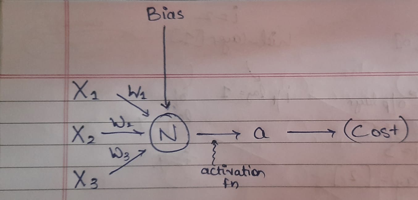
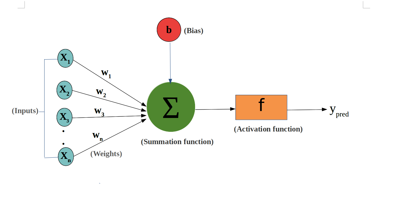
Lets take a good look at this above diagram. The Green circle is the Neuron.
Each Neuron has a bias (b), and a weights matrix($W \in \mathbb{R}^N$) which contain N number of values. N is the number of neurons in the previous layer. The math that happens before storing a value in the neuron is:

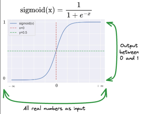
The $\sigma$ here is a sigmoid function. It is our activation function
This is a squishify function, which takes values from negative infinity to positive infinity and plots them between 0 and 1.
The idea is that each neuron will now store a scalar value.
Now lets talk about how to efficiently work on the summation of $\sum_{i=1}^{N} x_i W_i$. We know that X and W are stored in the form of matrices and both of them have N values. you could just take the dot product of X and W to get this summation. Remember to transpose one of them!

So essentially, each neuron stores a value calculates with the inputs given by all the neurons of the previous layer using the formula:

Also, remember the notation:

so we could also say,

2.2: Weights and Bias Indexing#

Notation:

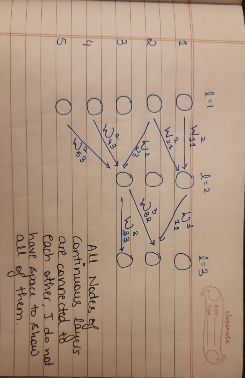
$W^{l}_{jk}$ is the weight representation.
Here:

• $l$ is the layer which the weight is going into.
• $j$ is the number of the neuron that info is being taken from in the $l^{\text{th}}$ layer.
• $k$ is the number of the neuron that info is being given to in the $(l-1)^{\text{th}}$ layer.

• $B^l_k$ is the representation for bias. Here:
• $l$ is the layer on the node
• $k$ is the numbering of that node in that layer. Sometimes, we have a singular bias for an entire layer $B^l$.

2.3 A layer of Neurons#

We know that all the Neurons store a singular scalar value. So, we just have a column matrix containing all the Neurons' values. The Neuron's value is called its Activation. The number of values in the column matrix will be the number of Neurons in that layer, $l$. Let us call this column matrix $S^l$, where $l$ corresponds to its layer.

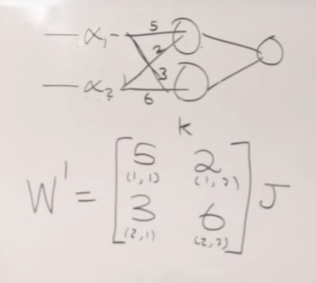
Lets talk about the storage of Weights matrix. We know that each Neuron will have a connection with all the previous layer's Neurons. This means: if the number of neurons in $(l-1)^{\text{th}}$ layer is $p$and the number of neurons in the $l^{\text{th}}$ layer is $q$. Then the number of values in the Weights matrix just for layer $l$ will be $(p \times q)$.

Now with this you could directly get the values of the $S^l$.

Now that you have $S^l$, you could do the same and find out $S^{(l+1)}$ by treating $S^l \text{ as } a^l$.

Part 3: Derivatives of Neural Networks#

3.1 Motivation and Cost Function#

You could imagine a machine with a lot of knobs. Each knob affects the final output by a certain amount. Keep in mind that some knobs affect the final output more than the others. Now how do you go about finding how each of these knobs change the final output and to what extent do they affect them?

That is what this entire section deals with.

Error Function:
The error function that we use here is MSE.

Keep in mind that the calculation of the loss is done in the Feedforward half of the NN. The gradient of the loss is done in the backpropagation half of the NN.

3.1.1 Derivation of a Binary element-wise operation#

A good place to start would be: What is a binary element-wise operation?
It is an operation which takes in two vectors and performs some element wise operation on them and gives out a singular vector.
This is a quick explanation as to why Jacobians here are always going to be diagonal matrices. Emphasis on the HERE, and by HERE, we mean when we are working with element wise functions.

Here we have a function F(v, w). It is a function which is undergoing a binary element-wise operation (+). Each row of F(v, w) is given names like $F_1, F_2, \ldots, F_n$.
Also, you need to keep note that $F_1$ contains $V_1$ and no other V's. Same with the other rows.

so now on differentiating, you can clearly observe why we get a diagonal matrix.

3.3.2 Derivative of a Hadamard Product#

A Hardmard Product is basically a binary element wise operation where we multiply 2 vectors element wise.

3.2.3 Derivative of a Scalar Expansion#

Let us take a quick look at how a computer solves this:

then multiplies it. This concept is called Broadcasting. Then depending on what the operation is, we get the derivative as before.

3.2.4 Derivative of a Sum#

where we are applying the function g(v) to every element then summing them up

Where: $S = \sum_{i} v_{i}$
hence we can clearly see that all of them will end up as 1.

3.3 Derivatives of a Neuron's Activation#

Now we will use all the above stuff:
Here is what we want to do:

We could rewrite this as:

Where $\oplus$ is the symbol for Hadamard product.
With the chain rule: keep in mind H = W $\oplus$ X and S = sum(H)

Lets work on the first the weights first:

Similarly using derivatives of sums:

And lets assume $\sigma$ is relu here because it makes out life easier and is more popular now.
Hence:

Now lets substitute all these values. We wont be assuming that $\frac{\partial a}{\partial Z}$ is 0, because that just cancels out everything.

Working this out:

Now if Z<0, then:

Working on bias now

We already calculated $\frac{\partial a}{\partial Z}$, and $\frac{\partial Z}{\partial b} = 1$, hence we get:
if Z>0

$\frac{\partial a}{\partial b} = 1$
if Z<0

3.4 Derivative of the cost for a simple neural network#

Here we use the MSE for the Loss function.

Before this we used to have inputs to a neuron. X, the neuron itself, which stored the weights W and the bias B. Using W, B and X, we get Z, passing it through an activation function, we get A.
Now we add onto this, and after we get A, we subtract it by the actual value we expect the neuron to get, $\hat{Y}$. Then we tend to normalize this error, using a tool like MSE or MAE(Mean absolute error). This is what we call the cost function. It is represented by $J(\theta)$.

Now that we know this, it shouldn't be too hard. Until now we had seen how the different aspects of a neuron like Z, or its activation function changes with respect to the weights and biases. Now we add onto that and see how the cost function changes with respect to the Weights and the Bias.

This is the final piece to the puzzle, the last link to the chain:

Now let us look at a dataset, We have the training examples as the columns and the feature numbers as the rows. Training example number will be shown by the superscript and the feature number as the subscript.

Now lets see how we can break down the last chain:

If we take $v = Y - \hat{Y}$. Then:

Now:

Where $a^L$ is the value we have got from the neural network.

Since Y is a constant.

The next step:

Now plug in the value of the derivative:

Now we considering the activation function is RelU and also value of Z is positive:

We get:

Substituting value of V:

Where $a^L = W^TX+b$. So the same thing as Z

if Activation function is RelU and value of Z is non positive:

3.5 Understanding the derivative of cost w.r.t weights#

Now Let us look at how this calculation is actually done:
Let us consider

Each training example has a different value of $e_i$.
Hence we get:

Now for simplicity sake, let us take m=1, and that training example has 5 features. And $e_i$ is the error of that training example:

Let us transpose this matrix so that it looks cleaner: (don't do it in the execution)

Now if we look closely, This is exactly how how cost changes with respect to each weight.

Let us now look at an example where we have M training examples:
Notations:

• $X^m_n$: Superscript is the training example, and the subscript is the feature number

That is:

The essence of this is very beautiful, Lets take a look at it:
Each row represents how much the error $J$ changes when we tweak that corresponding weight $W_1, W_2, W_3,...,W_n$.

In simpler words, it tells you how sensitive the cost function is to each of the weights to that neuron.

3.6 Differentiating the Bias#

Again lets take the chain rule and work on this:

Where $V = Y - a^L$.

We already know the value of

And also:

Now finding: $\frac{\partial J}{\partial V}$

We know that

And hence we get:

Substituting all the above values:

3.7 Gradient Descent Intuition#

Now that we have got the values for

For a single training example with 2 features.
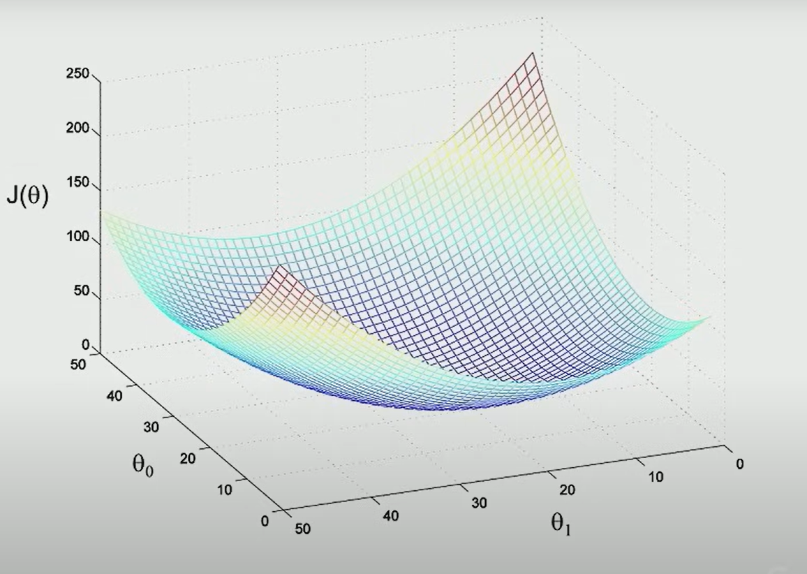
Imagine a huge blanket as such:

Then the gradient always points to the highest point of the blanket from any point.
Hence: Negative gradient points to lowest point of the blanket. The gradient is a vector of N dimensions pointing to the topmost point of the function.
So a more accurate way of representing the above function would be as such:

Where $\nabla_wJ$ is read as the gradient of J wrt W. It is a vector (2 dimensional here), pointing upward.
So With the gradient function, we could tell on changing which weight do we get the most bang-for-buck with respect to the cost function.
So each step needs to be in the direction of $-\nabla_wJ$ to reduce the overall loss.

3.8 Gradient descent algorithm and Stochastic Gradient Descent#

Now that we have the gradient of the cost function with respect to the weights and biases.

We can plug this into the traditional SGD algorithm:

Where $\theta$ is the weights vector, with each weights corresponding to the same differential in the gradient vector. $\alpha$ is the learning rate.

This is Gradient descent, what is Stochastic Gradient descent though?
Lets say we have a Training set of m = 10,000,000 training examples. Then we would have to calculate:

This would be painful to calculate, hence we break these down into batches, each of lets say.. 120 values. We then perform gradient descent over these batches. This would be computationally efficient. Now how do we stitch all of these batches values together. We just take one step per each batch. Remember to shuffle the training examples though.

3.9 Finding Derivative of an entire layer (and why it doesn't work the same way we did with one neuron)#

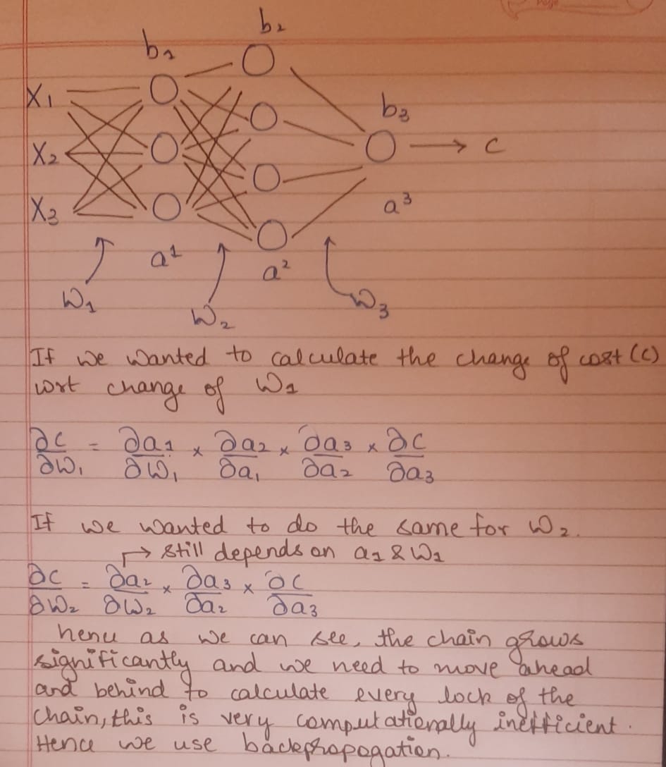
Here we shall delve deeper into why we do not use the forward pass to calculate the change of the cost with respect to the weights of the first layer, the second layer and so on.

The loss with respect to each node of a certain layer $l$ and a certain node of that layer $j$: $\delta_{j}^{l}$

Now why is backpropagation better?
Backpropagation makes sure you calculate all the values, including C, then we move backwards. By backwards, we calculate: $\frac{\partial C}{\partial a_{3}}$.

We store this value as we will need it later too.
Then we move a step back to calculate how the weight of the node $W_{1}^{2}$ affects Cost. This is going to be:

Now we just use the previously stored value and get this answer easily.

Part 4: Backpropagation#

4.1: The error of a Node#

Let us get some notations clear before getting started with this:

• $\delta_{j}^{l}$:The error of the $j^{th}$node of the $l^{th}$ layer,
• $Z_{j}^{l}$:The Z of the $j^{th}$ node of the $l^{th}$ layer.
• $\Delta$: The small change made to Z.

We know that:

When we want to make a small change to this activation, we do not mess with the activation as a whole instead we add a small change to Z.

Then pass it through the activation function. And then we calculate the error of the node:

Why does this make sense though?
This is because if the value of error of the node is tiny, then on changing the node's parameters will not change the cost to a high extent. On the other hand, if it were high, that would mean, on changing the parameters of the node, we could drastically reduce the cost. Basically the same bang-per-buck idea.

4.2 The Four Equations of Backpropagation#

4.2.1 Equation 1: Finding the error of all nodes in the last layer#

Lets take a neural network with L layers.

Where $a^{L}_{j} = \sigma(Z^L_{j})$. So the second link to the chain is just the derivative of the activation function we choose to use.

This is now the error of the $j^{th}$ node of the $L^{th}$ layer. Let us vectorize this and write it down for the entire layer $L$, which has $J$ nodes.

On observing closely, This is just the gradient vector of the cost with respect to the activation of the $L^{th}$ layer multiplied with the derivative of the activation function of Z of that node.

This is possible to calculate for the last layer, because we already have the values of the expected outputs (The labels of the model). So we use this as the layer that comes after the last hidden layer and calculate the error of the Lth layer.

4.2.2 Equation 2: Finding the error of any node#

With this equation, if we know the error of the $(l+1)^{th}$ layer,$\delta^{l+1}$. Then we can find the error of the $l^{th}$ layer, $\delta^l$.

That is, if we take the dot product of the weights matrix of the $(l+1)^{th}$ and its errors. Then we element wise multiply it with the derivative of the activation function of the $l^{th}$ layer, we get the $l^{th}$layer errors.

Keep in mind that:

• The weights matrix of a layer is of dimensions (input size x output size)
• The error of a layer is a vector of J elements (where J is the number of neurons in that layer)
• $\sigma'(Z^l)$ is a vector of J elements where J is the number of neurons in the layer.

Hence using this simple equation, we could just backpropagate and get the activations for all the layers.

4.2.3 Equation 3: Finding the derivative of the cost w.r.t any bias#

The derivative of cost with respect any bias is given by the:

Now we could just use the chain rule again to get this:

But,

Hence,

4.2.4 Equation 4: Finding the derivative of the cost w.r.t any Weight#

For the derivation, let us take 2 layers. The $(l-1)^{th}$ and the $l^{th}$ layers. Let take the weight going from the $k^{th}$neuron to the $j^{th}$ neuron of the previous to the next layer respectively.

With the chain rule:

The second term here is the error of the node. $\delta_{j}^l$

We only need the first term:

Putting all the pieces together we get:

4.2.5 Finding the derivative of the cost w.r.t any Weight VECTORIZED#

Using the formula that we derived above, we can transform the weights matrix into a derivative.
As we know, the weights matrix for a neural network which has $j$ neurons in the $l^{th}$ layer. and $k$neurons in the $(l-1)^{th}$ layer.

Using the above formula, we get the element wise cost function derivation. Do not confuse this for matrix differentiation, which is completely different.

But there is another way to show this, which includes the dot product of 2 vectors, but its slightly different, here's how:

Now multiply these such that you get a $(j \times k)$ matrix. You will get the same thing as above.

So we could say:

4.3 Tying Part 3 and Part 4 together (The two ways of calculating derivatives)#

We have derived 4 important formulae:
From the feed-forward half:

From the backpropagation:

We also know that: we could just write

Hence, we could rewrite the feedforward half as:

Now for the sake of simplicity, let us take just one training example:
Hence:

Now do these ring a bell? They are the exact same formula we got for the backpropagation algorithm:

4.4 The Backpropagation Algorithm#

Backpropagation formulae:

Here are the steps we follow in a neural network:

• During forward propagation, we calculate $a^L$s and $Z^l$s.
• Compute the cost
• Use the first formulae to get the error of the last layer. $\delta^L$
• Now use the second equation to get the rest of they layer's errors. $\delta^l$
• Use third equation to get the bias derivatives
• Use fourth equation to get the weight derivatives

Some other tips to build your NN:

• Each layer must also have a derivative of the weights matrix as shown above in section 4.2
• Each layer must have a derivative of the biases vector as shown above
• Then make sure to concatenate these 2 vectors after flattening the weights vector. This gives you your $\theta$ vector
• Use this $\theta$ and apply gradient descent on it.

Source