Attention is all you need!

• Get the dataset you want to train your model on.

  • !wget <https://raw.githubusercontent.com/karpathy/char-rnn/master/data/tinyshakespeare/input.txt
  • read the data:
    • with open('input.txt', 'r', encoding='utf-8') as f:
      • text = f.read()
  • Now text is a long string containing all the data from the dataset.

• Take a good look at your dataset and also observe how you could tokenize your data.

• Define a few necessary hyperparameters like vocab_size, which contain the number of chars in the sequence text and chars containing all the unique characters, this is very important as we are building a character based model, that is, each character is a token.

  • chars = sorted(list(set(text)))
  • vocab_size = len(chars)

• Tokenize your dataset. Here, since we are working on a character based model, each unique character is given a unique integer and mapped to it. char_to_int and int_to_char will be our two maps. The first to encode and the second to decode.

  • Dictionary to go from char to int: stoi = {ch:i for i, ch in enumerate(chars)}
  • Dictionary to go from int to char: itos = { i:ch for i,ch in enumerate(chars)}
  • function to encode: encode = lambda s: [stoi[c] for c in s]
  • function to decode: decode = lambda l: ''.join([itos[i] for i in l])

• Now that we have the functions to encode and decode our text, we can go ahead and encode the whole text.

  • You need to encode it and store the data in a torch tensor. So we need to import torch
    • import torch
  • Now you could encode it and store it in data:
    • data = torch.tensor(encode(text), dtype = torch.long)

• Divide your dataset into training and validation sets. All further work will include working on only the training dataset. In this model we choose to use a 90:10 split for train and validation.

  • split_fraction = 0.9
  • n = int(split_fraction * len(data))
  • train_data = data[:n]
  • val_data = data[n:]

• Set your hyperparameters:

  • block-size - size of each chunk of data you're sending to the compute at a time.
    • block_size = 8
  • batch-size - number of chunks of data you will process parallelly
    • batch_size = 4

• Now that you have your hyperparameters, let us work on making features and labels out the data we have.

  • Features
    • Pick batch-size number of random indices on the data and using those indices get block-size number of continuous values and stack them on top of each other. This gives you your features vector.
    • Since we are stacking them on top of each other, we end up with a tensor of dimensions (batch-size* , *block-size) for our features vector.
  • Labels
    • In the model we are working on, we take all the previous characters in the batch and these are the features/context. As for labels, we take the character right after the features/context. This is how we get out labels vector. As for the labels vector, we again stack them up as we did for the features vector.
    • As explained we end up with a tensor of dimensions (batch-size, block-size) for our labels vector.
  • Code of the above:
    • We make a function which takes in the type of split you want to put into batches and blocks. split is a string that takes in whether the split you want to work on is the train split or the test split.
      • def get_batch(split):
    • We then get the data we are going to splitting into batches and blocks depending on split.
      • data = train_data if split == "train" else val_data
    • We can now work on constructing the features array.
      • x = torch.stack([data[i:i+block_size] for i in ix])
    • Similarly the labels array.
      • y = torch.stack([data[i+1:i+block_size+1] for i in ix])
    • Then return the values we have calculated.
      • return x, y
  • We can now get batches and blocks from either the train_data or the val_data. Here i am going to take a batch from the train_data:

    • xb, yb = get_batch('train')

    • xb and yb now look somewhat like this: both are of dimensions (batch_size = 4, block_size = 8)

      • xb =
      textCopy

      tensor([[24, 43, 58, 5, 57, 1, 46, 43],
              [44, 53, 56, 1, 58, 46, 39, 58],
              [52, 58, 1, 58, 46, 39, 58, 1],
              [25, 17, 27, 10, 0, 21, 1, 54]])

      • yb =
      textCopy

      tensor([[43, 58, 5, 57, 1, 46, 43, 39],
              [53, 56, 1, 58, 46, 39, 58, 1],
              [58, 1, 58, 46, 39, 58, 1, 46],
              [17, 27, 10, 0, 21, 1, 54, 39]])

    • We can observe that, when {24} is the context(at xb), we have target(at yb) as {43}, which is the next element in xb's first batch. When we have {24, 43} as the context, we have {58} as the target, and so on. We can also observe that when we have {24, 43, 58, 5, 57, 1, 46, 43} as the context, we have {39} as the target which comes right after the sequence of context in the train_data but is not quiet visible to us in xb.

• Visualizing all that we have done till now:

  • train_data[:block_size + 1]
  • we have (block_size + 1) because we want to see the target when we have all eight values as context.
  • Output:
  textCopy

  tensor([18, 47, 56, 57, 58,  1, 15, 47, 58])

  • In this block,
    • when input is tensor([18]) the target: 47
    • when input is tensor([18, 47]) the target: 56
    • when input is tensor([18, 47, 56]) the target: 57
    • when input is tensor([18, 47, 56, 57]) the target: 58
    • when input is tensor([18, 47, 56, 57, 58]) the target: 1
    • when input is tensor([18, 47, 56, 57, 58, 1]) the target: 15
    • when input is tensor([18, 47, 56, 57, 58, 1, 15]) the target: 47
    • when input is tensor([18, 47, 56, 57, 58, 1, 15, 47]) the target: 58
  • This is the same for each block.
  • We implemented the same and made out features and labels vectors.

• We can now get started with building the model.

  • We now need a tensor of size (vocab_size, vocab_size). This is going to be called the token_embedding_table. We initialize it in the constructor of the BigramLanguageModel subclass, which is an extension of the nn.Module class.
  • class BigramLanguageModel(nn.Module):
  • We also need the following libraries:
  • import torch
  • import torch.nn as nn
  • from torch.nn import functional as F
    • constructor which takes the vocab_size as a parameter
      • super().__init__() because it is a daughter class
      • self.token_embedding_table = nn.Embedding(num_embeddings = vocab_size, embedding_dim = vocab_size)
        • This defines an embedding table and initializes it with random values.
  • We also define a special function in Pytorch called forward().
    • def forward(self, idx, targets = None) idx is the features vector we calculated earlier, targets is the labels vector we calculated earlier.
    • This function basically tells the neural network what activation function to apply as we pass data along the layers. It is automatically called whenever we create an object of the same class and initialize the object. So, in simple terms, when we create and initialize an object, we automatically call the constructor and the forward functions.
  • To the forward() function. We pass the features and the labels. We then calculate the logits. logits is a vector of (B, T, C) dimensions. B stands for batch, T stands for time and C stands for channel. I shall explain this working in great detail.
    • We import the torch.nn library as nn
    • We then make an object of the class nn.Embedding. We are going to call this object the token_embedding_table. While making this object we need to pass 2 arguments to the constructor of the nn.Embedding class. These arguements are:
      • num_embeddings --> the number of unique token we have in the dataset
      • embedding_dim --> c value. This defines how we want to store the data of each token. When we say data of each token, we refer to the connections of this token with the other tokens in the same batch. We can choose a high number for C. This would increase the clarity of the connections between the different tokens, but at the same time, it would increase computation time. It we used a small number for C, this would mean the computation time would be lesser, but, the clarity in the connections between tokens would be smaller.
    • At the constructor, it initialized random values in all the cells of the token_embedding_table.
    • When the forward() function runs, it takes in the features vector, and passes this as the argument to the object of the nn.Embedding class. That is, the token_embedding_table. logits = self.token_embedding_table(x) takes in the features vector and makes a table of (B, T, C) with the (B, T) table we have seen in the form of features vector. It just extends each of these cells of the (B, T) table and makes it store information in C amount of cells right behind it.
    • The main takeaway is that, it takes in the features table and then makes sure that every token in the features table has C number of cells which store it's information with respect to other tokens in the same batch.
    • We now need to evaluate the loss. A good way of measuring the loss is the negative log likelihood. This is done using an inbuilt function called the cross_entropy. To use cross_entropy:
      • We need to import from torch.nn import functional as F
      • We will need to reshape the logits and targets so make sure to preserve the shape B, T, C = logits.shape
      • We also need to reshape the logits because cross_entropy expects a 2d array, with the first dimension containing tokens and the second containing channels. That is it wants a (B x T , C) dimension features array and a (B x T) dimension labels array. So we run the commands logits = logits.view(B*T, C) targets = targets.view(B*T, C) (view is basically reshape, but when using tensors, view is more reliable).
      • Then we get the loss by loss = F.cross_entropy(logits, target)
    • The forward() function returns loss and the logits.
    • Generating output: def generate(self, idx, max_new_tokens):
      • idx is the features vector, max_new_tokens is the maximum number of tokens you want the model to generate.
      • The generate function takes in idx (A (B x T) array and makes that a (B x T+1), then a (B x T+2) array and so on till it becomes (B x max_new_tokens).
      • We loop around max_new_tokens times to produce each token at a time. for _ in range(max_new_tokens)
        • This just means that, initially, we have idx as the context/features. we guess the next token (a char) then, during the next iteration of the loop, it takes the old context and the next token as the new context/features to make a new guess. this keeps happening until the loop terminates
        • Inside the for loop, we first get the logits and the loss for the initial idx that was submitted to the generate() function as context. logits, loss = self(idx)
        • Now we alter the logits. We only take into consideration the channels and the batches of the last target. That is, we only want the part of the context that will be used to give predictions. We only take the last row of the time section while retaining all of the last row's channels and batches. logits = logits[:, -1, :]
        • We then use Softmax as a matrix trimming method. Matrix trimming is a wide topic which i shall discuss soon. prob = F.softmax(logits, dim = -1)
        • Now that we have the probabilities of the next character's pick from the bucket of tokens. We pick an index of the token from the bucket of tokens keeping in mind the probability of each token occurring with respect to the context provided. torch provides a very helpful function to do the same. idx_next = torch.multinomial(prob, num_samples = 1)
        • This above code tells the torch library, now that we have given the probability of each token ouccering in the bucket of tokens, pick num_of_samples (an int) to give. The output is going to be an index, which here could just be converted to char by using the encode and decode functions we defined earlier.
        • Then we just concatenate the idx_new to idx idx = torch.cat((idx, idx_new), dim = 1) Then we end the loop.
      • Outside the loop, we return the idx value that we have concatenated to. During input, idx was (B x T), now during the termination of the function generate(), it is of size (B x T + max_new_tokens)
        • return idx

• To make use of the code we have written above, you make an instance/object of this class m = BigramLanguageModel(vocal_size)

• Get the logits and loss logits, loss = m(xb, yb)

• Now we are ready to get out first output:

  • We are basically going to create a (B x T) array of (1 x 1) which has a zero. We then send it to the generate() function and generate 100 new tokens.
    • idx = torch.zeros((1, 1), dtype=torch.long)
    • print(decode(m.generate(idx, max_new_tokens=100)[0].tolist()))
  • Output looks somewhat weird now:
    • Sr?qP-QWktXoL&jLDJgOLVz'RIoDqHdhsV&vLLxatjscMpwLERSPyao.qfzs$Ys$zF-w,;eEkzxjgCKFChs!iWW.ObzDnxA Ms$3
  • Lets look at why this is happening. Our model now is a typical Bigram model. This type of model only looks at the previous token (which is a char here) as context. Using this context, it predicts the next char. What we actually need to be doing is looking at all of the char before the prediction char and then predict a char. Lets work on that.

• Lets first choose an optimizer. Our best bet for this model is AdamW. This optimizer is not too simple, its not too complex and gets the job done well.

  • optimizer = torch.optim.AdamW(m.parameters(), lr=1e-3)

• Also before we make use of this optimizer, let us get the batch_size up to a more reasonable value. We can be doing way more calculations in parallel.

  • batch_size = 32

• Let us also define the number of epochs we want to run.

  • An epoch is basically the number of times we run through every example of the whole dataset.
  • epochs = 1000

• Now we can explain what we do in every iteration of every epoch

• for steps in range(epochs):

  • sample a batch of data using the get_batch(split) function we made earlier.
    • xb, yb = get_batch('train')
  • Generate the loss
    • logits, loss = m(xb, yb)
  • Set the gradients from previous iteration to zero
    • optimizer.zero_grad(set_to_none=True)
  • Get the gradients for all the parameters
    • loss.backward()
  • Use these gradients to update parameters
    • optimizer.step()
  • This is the end of the for loop

• Now we can try to get the output again:

  • print(decode(m.generate(idx = torch.zeros((1, 1), dtype=torch.long), max_new_tokens=300)[0].tolist()))
  • Output looks like:
    • Iyoteng h hasbe pave pirance Rie hicomyonthar's Plinseard ith henoure wounonthioneir thondy, y heltieiengerofo'dsssit ey KIN d pe wither vouprrouthercc. hathe; d! My hind tt hinig t ouchos tes; st yo hind wotte grotonear 'so it t jod weancotha: h hay.JUCle n prids, r loncave w hollular s O: HIs; ht

• This looks significantly better then the previous output.

• MATHEMATICAL TRICK IN SELF ATTENTION

  • We want to work on a mathematical trick that helps us make a lower triangular matrix where each row elements adds up to 1.

    • For example:

      • from input tensor:
      textCopy

      tensor(
        [1,2,5,7],
        [1,1,1,9],
        [1,1,1,1],
        [0,1,4,5]
       )

      • to output tensor:
      textCopy

      tensor(
       [1,   0,   0,   0], --> adds up to 1
       [0.3, 0.7, 0,   0],-->  adds up to 1
       [0.1, 0.1, 0.8, 0], --> adds up to 1
       [0.7, 0.1, 0.1, 0.1] ) --> adds up to 1

  • We do this for a very specific reason. In the (B, T, C) array we had. You could recall that we had a batch, time matrix and the each value corresponding to the cell in this matrix stored values about that corresponding token's relations with the other tokens in the same column (that is, the same batch). We have details of the token's relations with the previous tokens and the next tokens in the same batch. In this model, we only want it to store relations of that token with the previous tokens and not the latter tokens. This is because the latter tokens are to come in the future and they haven't been predicted yet. So, in simple terms, the numbers per column are just the connections to the previous tokens, and it is in the form of a probability, meaning, we want it to add up to one.
  • We have 3 methods of matrix trimming explained in the video, but I am just going to use the third method.
  • METHOD 3:
    pythonCopy

    xbow3 = torch.zeros((B,T,C))
    tril = torch.tril(torch.ones(T, T))
    wei = torch.zeros((T,T))
    wei = wei.masked_fill(tril == 0, float('-inf'))
    wei = F.softmax(wei, dim=-1)
    xbow3 = wei @ x

• In simple terms, each token in the (B, T) array emits 3 values, a Query, Key and Value. Query is what the token is looking for and the Key is the the array telling us what the token is. We now take each Query and then dot product it with each Key of that batch. This gives us the Weights matrix which we call wei. Now lets say the Query and the Key align very well. As in the connection between those two tokens is very high, then they tend to interact drastically. This gives us a huge value in the wei matrix. Value is the array that each token emits which tells us in detail what each token contains. To sum it all up, in perspective of the token:

  • Query --> "what am i looking for?"
  • Key --> "What does this token mean?"
  • Value --> "What information does this token convey?"
    • Imagine you going to a book store. What kind of book you're looking for is the Query, The book's title or the front page is the Key and the contents of the book is the Value.
    • So Value of the token is only comes into play when the interaction between the Key and the Query is good.
  • Weight --> "How well does this token interact with the other tokens?"

• In this code block we are initializing 3 simple neural networks called key, query and the value.

  pythonCopy

  head_size = 16
  key = nn.Linear(C, head_size, bias=False)
  query = nn.Linear(C, head_size, bias=False)
  value = nn.Linear(C, head_size, bias=False)

• Let us talk about the nn.Linear neural network.

  • This is a neural network that takes in Number of input features, Number of output features and Bias(true or false) to initialize.
  • This basically performs the operation: Y = X . W$^T$+ b
  • Lets say we initialize the layer with the number of input features as 3, the number of output features as 1 and the bias as True.
    • torch.nn.Linear(3,1,True)
  • Now we are set to give this layer input data and the layer will perform the operation as mentioned above and give out a singular output value for each training example.

  • In this example, let us take the number of training examples as 2. So we get an X matrix like below:#

    $$\left| \begin{matrix} 1 & 2 & 3 \\ 2 & 4 & 1 \end{matrix} \right|$$

  • Now our weight matrix W looks somewhat like this (It is randomly initialized by pytorch):#

    $$W = \left| \begin{matrix} -0.020 & 0.5852 & -0.2880 \end{matrix} \right|$$

  • And our Bias will also be randomly initialized singular value on a 1 x 1 matrix.#

    $$Bias = \left| 0.5594 \right|$$

  • Here is how our calculation takes place:#

    $$Y = X W^T + \text{Bias}$$
    • Since, the dot product of X and W are of dimensions (2 x 1), bias also is made into a (2 x 1) matrix.
    $$Y = \left| \begin{matrix} 1 & 2 & 3 \\ 2 & 4 & 1 \end{matrix} \right|  \cdot  \left| \begin{matrix} -0.020 \\ 0.5852 \\ -0.2880 \end{matrix} \right|  +  \left| \begin{matrix} 0.5594 \\ 0.5594 \end{matrix} \right|$$
    $$Y = \left| \begin{matrix} 0.2414 \\ 1.4072 \end{matrix} \right|$$
    • This is the output.
  • Each training example gives in N number of features and gets M number of outputs. This operation could be done with or without bias.

• So now coming back to the Key, Query and Value neural networks. Key, Query and Valueare 3 neural networks that takes in C number of features and converts it into head_size number of values(that is 32 to 16).

• Now we pass in the x to the key and the query neural networks.

  • k = key(x)
  • q = query(x)

• So now, k is a (B, T, 16) array, where each token of the (B, T) matrix contains a 16 cell array as its key. Similarly, q is a (B, T, 16) array, where each token of the (B, T) matrix contains a 16 cell array as its query.

• Now we can dot product each of the token's keys and queries to get the weights, that is the wei array.

  • wei = q @ k.transpose(-2, -1)

• wei array is a (B, T, T) array.

• Now we use the MATHEMATICAL TRICK IN SELF ATTENTION. We know that the 3rd method is the best method to do this. Hence we choose it.

  • tril = torch.tril(torch.ones(T, T))
  • wei = wei.masked_fill(tril == 0, float('-inf'))
  • wei = F.softmax(wei, dim=-1)

• This gives us wei.

• Now we take the dot product of the wei and Value:

  • v = value(x)
  • out = wei @ v

• We also multiply the wei by sqrt(head_size). This is done to keep variance of it at 0.

• wei = wei * head_size ** 2

• If we don't do this, we would end up with vectors that have variance of the order of head_size. This is an issue because if we we have a variance of order head_size, then we end up with a vector that looks pretty similar to a one hot vector. This is bad because then we would be taking information from a singular place instead of multiple tokens of the sentence.

• Now lets just convert this into script code (a .py file from a .pynb file):

import torch
import torch.nn as nn
from torch.nn import functional as F
# hyperparameters
batch_size = 16 # how many independent sequences will we process in parallel?
block_size = 32 # what is the maximum context length for predictions?
max_iters = 5000
eval_interval = 100
learning_rate = 1e-3
device = 'cuda' if torch.cuda.is_available() else 'cpu' # New: explained after code block
eval_iters = 200 # New: explained after code block
n_embd = 64 # New: explained after code block
n_head = 4
n_layer = 4
dropout = 0.2 # Explained in detail in the Dropout section of the cleaning up the code.
# ------------
torch.manual_seed(1337)
# getting the data and then reading it
# wget <https://raw.githubusercontent.com/karpathy/char-rnn/master/data/tinyshakespeare/input.txt>
with open('input.txt', 'r', encoding='utf-8') as f:
    text = f.read()
# here are all the unique characters that occur in this text
chars = sorted(list(set(text)))
# finding the number of unique chars in the chars
vocab_size = len(chars)
# create a mapping from characters to integers
stoi = { ch:i for i,ch in enumerate(chars) }
itos = { i:ch for i,ch in enumerate(chars) }

encode = lambda s: [stoi[c] for c in s] # encoder: take a string, output a list of integers
decode = lambda l: ''.join([itos[i] for i in l]) # decoder: take a list of integers, output a string

# Train and test splits
data = torch.tensor(encode(text), dtype=torch.long)
n = int(0.9*len(data)) # first 90% will be train, rest val (split_fraction)
train_data = data[:n]
val_data = data[n:]

# making batches (features and labels) out of the said data split type (train or validation)
def get_batch(split):
    # generate a small batch of data of inputs x and targets y
    data = train_data if split == 'train' else val_data
    ix = torch.randint(len(data) - block_size, (batch_size,))
    x = torch.stack([data[i:i+block_size] for i in ix])
    y = torch.stack([data[i+1:i+block_size+1] for i in ix])
    x, y = x.to(device), y.to(device) # NEW: Explained after code block
    return x, y

@torch.no_grad()

# calculates the loss and the logits for the specified model and then gives it out
def estimate_loss():
    out = {}
    model.eval() # Setting model to evaluation phase
    for split in ['train', 'val']:
        losses = torch.zeros(eval_iters) # An array of zeroes of size eval_iters
        # this loop just counts indices from 0 to eval_iters-1 and then fills in the losses of the batches in the losses array.
        for k in range(eval_iters):
            X, Y = get_batch(split)
            logits, loss = model(X, Y)
            losses[k] = loss.item()

        out[split] = losses.mean()

    model.train() # resetting it back to training phase
    return out # an array of 2 float containing the mean of all the losses of training and validation phases calculated over eval_iters number of batches

class Head(nn.Module):
    """ one head of self-attention """
    def __init__(self, head_size):
        super().__init__()
        # Getting the key, query and the value as mentioned previously.
        self.key = nn.Linear(n_embd, head_size, bias=False)
        self.query = nn.Linear(n_embd, head_size, bias=False)
        self.value = nn.Linear(n_embd, head_size, bias=False)
        # register_buffer ensures it is not affected by optimizer.step()
        self.register_buffer('tril', torch.tril(torch.ones(block_size, block_size)))
        self.dropout = nn.Dropout(dropout) # explained in cleaning up of code (dropout).

    def forward(self, x):
        B,T,C = x.shape
        k = self.key(x)   # (B,T,C)
        q = self.query(x) # (B,T,C)
        # compute attention scores ("affinities")
        wei = q @ k.transpose(-2,-1) * C**-0.5 # (B, T, C) @ (B, C, T) -> (B, T, T)
        wei = wei.masked_fill(self.tril[:T, :T] == 0, float('-inf')) # (B, T, T)
        wei = F.softmax(wei, dim=-1) # (B, T, T)
        wei = self.dropout(wei) # explained in cleaning up of code (dropout)
        # perform the weighted aggregation of the values
        v = self.value(x) # (B,T,C)
        out = wei @ v # (B, T, T) @ (B, T, C) -> (B, T, C)
        return out

# super simple bigram model
class BigramLanguageModel(nn.Module):
    def __init__(self):
        super().__init__()
        # each token directly reads off the logits for the next token from a lookup table
        self.token_embedding_table = nn.Embedding(vocab_size, n_embd)
        self.position_embedding_table = nn.Embedding(block_size, n_embd)
        # interspacing communication multiple times.
        self.blocks = nn.Sequential(*[Block(n_embd, n_head=n_head) for _ in range(n_layer)])
        self.ln_f = nn.LayerNorm(n_embd) # final layer norm
        self.lm_head = nn.Linear(n_embd, vocab_size) # language modelling head

    def forward(self, idx, targets=None):
        B, T = idx.shape
        # idx and targets are both (B,T) tensor of integers
        tok_emb = self.token_embedding_table(idx) # (B,T,C)
        pos_emb = self.position_embedding_table(torch.arange(T, device=device)) # (T,C)
        x = tok_emb + pos_emb # (B,T,C)
        x = self.blocks(x) # (B,T,C)
        x = self.ln_f(x) # (B,T,C)
        logits = self.lm_head(x) # (B,T,vocab_size)

        if targets is None:
            loss = None
        else:
            B, T, C = logits.shape
            logits = logits.view(B*T, C)
            targets = targets.view(B*T)
            loss = F.cross_entropy(logits, targets)

        return logits, loss

    def generate(self, idx, max_new_tokens):
        # idx is (B, T) array of indices in the current context
        for _ in range(max_new_tokens):
            # crop idx to the last block_size tokens
            idx_cond = idx[:, -block_size:]
            # get the predictions
            logits, loss = self(idx_cond)
            # focus only on the last time step
            logits = logits[:, -1, :] # becomes (B, C)
            # apply softmax to get probabilities
            probs = F.softmax(logits, dim=-1) # (B, C)
            # sample from the distribution
            idx_next = torch.multinomial(probs, num_samples=1) # (B, 1)
            # append sampled index to the running sequence
            idx = torch.cat((idx, idx_next), dim=1) # (B, T+1)
        return idx

model = BigramLanguageModel()
m = model.to(device) # New: explained after code block
# print the number of parameters in the model
print(sum(p.numel() for p in m.parameters())/1e6, 'M parameters')
# create a PyTorch optimizer
optimizer = torch.optim.AdamW(model.parameters(), lr=learning_rate)
for iter in range(max_iters):
    # every once in a while evaluate the loss on train and val sets
    if iter % eval_interval == 0 or iter == max_iters - 1:
        losses = estimate_loss()
        print(f"step {iter}: train loss {losses['train']:.4f}, val loss {losses['val']:.4f}")
    # sample a batch of data
    xb, yb = get_batch('train')
    # evaluate the loss
    logits, loss = model(xb, yb)
    optimizer.zero_grad(set_to_none=True)
    loss.backward()
    optimizer.step()

# generate from the model
context = torch.zeros((1, 1), dtype=torch.long, device=device) # New: explained after code block
print(decode(m.generate(context, max_new_tokens=2000)[0].tolist()))

• Key differences between the .ipynb notebook and the .py file here is:
• A few new parameters:
• device : this parameter tells the device to run on a gpu if you have got one on your system. Could be either cuda or could be cpu.
• If device == 'cuda': then we also need to move the model, the batches to gpu as well. When generating output, we also need to specify the device as well.
• The get_estimate() function averages up the loss over multiple batches. It averages eval_iters number of batches' average. This is done for both training and validation data. This is way less noisy as the previous one. It basically prints the loss as before but only once every eval_iters number of batches have passed, by averaging out the last eval_iters number of batches' loss.
• We also do not need to pass vocab_size since it is a global variable to the constructor of the class BigramLanguageModel.
• We also introduce the hyperparameter n_embd which stands for the number of parameters and instead of defining the embedding table with (number of tokens = vocab_size, number of simensions(c) = vocab_size), we define it with (number of tokens = vocab_size, number of dimensions(c) = n_embd).
• Adding to the above code:
• Now we shall implement the MultiHeadAttention(nn.Module). As per documentation, this is basically running multiple heads of SelfAttention parallelly. Then we concatenate the heads at the end.

class MultiHeadAttention(nn.Module):
    """ multiple heads of self-attention in parallel """
    def __init__(self, num_heads, head_size):
        super().__init__()
        # defining a list of all layers of the neural network. We use this instead of a python list because pytorch can analize this in real time unlike in a python list. This list now contains num_heads number of items. where for each cell we call the Head class and pass it head_size for its constructor.
        self.heads = nn.ModuleList([Head(head_size) for _ in range(num_heads)])
        # for residual connections(explained later)
        self.proj = nn.Linear(n_embd, n_embd)
        self.dropout = nn.Dropout(dropout) # explained lated under cleaning up the code

    def forward(self, x):
        # concatenating to the list.
        out = torch.cat([h(x) for h in self.heads], dim=-1)
        out = self.dropout(self.proj(out))
        return out

• Quickly explaining the above code block:
• We are creating a daughter class called MultiHeadAttention(nn.Module) of the parent class nn.Module.
• We also earlier created a hyperparameter called num_heads. This is the number of heads we are going to run in parallel. So now instead of sending it 32 number of tokens per batch at once, we can just send 32 / 4 = 8 tokens and then say we want to process 4 of them parallelly and then just concatenate the 4 results of heads at the end and then we would still end up with the same output as before.
• Now we can implement the FeedForward part to our transformer. This is done to improve the working of the model. Until now, all the models we have used are linear. This is a huge issue. As the entire model is a massive Linear function without a FeedForward. We do not want that. We want it to also be able to take in non linear functions into play. This is exactly what FeedForward does.
• How does it introduce Non-linearity? It uses activation functions like RelU and Leaky-RelU.
• So initially if we had a neural network that did

meaning it would give output like this:

Now after adding the FeedForward network:

Meaning it would give outputs as such:

 class FeedFoward(nn.Module):
    """ a simple linear layer followed by a non-linearity """
    def __init__(self, n_embd):
        super().__init__()
        self.net = nn.Sequential(
            nn.Linear(n_embd, 4 * n_embd),
            nn.ReLU(),
            nn.Linear(4 * n_embd, n_embd),
            nn.Dropout(dropout),
        )

	def forward(self, x):
        return self.net(x)

• Now we can introduce the Block. This is basically an amalgamation of all The entire transformer architecture. Here we are basically connecting all the dots and connections for all the other parts of the architecture that we have worked on till now.

class Block(nn.Module):
    """ Transformer block: communication followed by computation """
     def __init__(self, n_embd, n_head):
        # n_embd: embedding dimension, n_head: the number of heads we'd like
        super().__init__()
        head_size = n_embd // n_head # explained in first point
        self.sa = MultiHeadAttention(n_head, head_size) # Self attention
        self.ffwd = FeedFoward(n_embd) # calling of the feedforward class
        self.ln1 = nn.LayerNorm(n_embd) # explained in LayerNorm
        self.ln2 = nn.LayerNorm(n_embd)  # also explained in LayerNorm

	def forward(self, x):
		# residual connections by using x = x + (deviated value)
		# LayerNorm by altering deviated value by (self.sa(self.ln1(x))) before the Self attention and altering deviated value by (self.ffwd(ln2(x))) before the FeedForward sections. Not similar to the architecture diagram below as we are implemeting LayerNorm before FeedForward as in case of ln1 and before Self Attention in case of ln2.
        x = x + self.sa(self.ln1(x)) # residual connections and LayerNorm
        x = x + self.ffwd(self.ln2(x)) # residual connections and LayerNorm
        return x

• head_size = n_embd // n_head This is basically the implementation of the MultiHeadAttention as explained above.

• Now that we have this, we have a proper working model of the transformer. But, this is now a deep neural network, which has a few optimization problems, let us take a look at how to set that right. We have two methods we are implementing here:

• Residual connections:

  

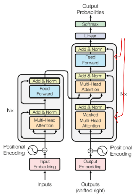
• The two connections shown above are the residual connections in the transformer architecture. In very simple terms it is a highway where the information is stored and then any changes made by the FeedForward section will be added to the highway, as opposed to just changing the value each iteration of the FeedForward. Initially the Residual connections do not provide much info on the highway. As the optimization goes on, we would see a drastic rise in the contributions of the Residual connections and decrease in the contributions of the FeedForward block.

• So we fork off the highway and do computations through the FeedForward network and then rejoin the highway.

• LayerNorm(Not implemented in my .ipynb notebook):

  

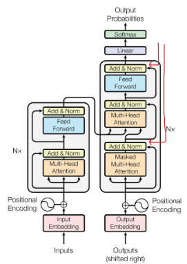
• These Red lines point to the LayerNorm on the Transformer architecture. We want to normalize rows instead of columns here.

• The above architecture is pretty old, nowadays we apply the Add & Norm before the FeedForward. We have implemented the newer version of this. See how we in the above code block we have applied it on x before sending it to the Self attention and the FeedForward sections.

• Cleaning up code:

  • We introduce two new hyperparameters n_layers and n_heads that specifies the number of new layers we have and the number of heads respectively.
  • Added Dropout. It is basically something you add right as the deviation from the separated path (Residual connection reference) joins the highway again.
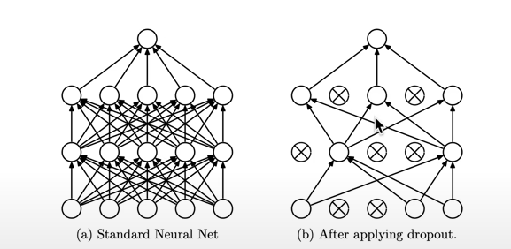
    • Dropout in very simple terms shuts off some random nodes of the neural network from communicating to the next nodes.

      

• This is very helpful because when we randomly shut off a few nodes, we get multiple subnetworks trained. In the end we just put all of these subnetworks together to make a way more robust neural network.

• It works as a regularization technique and helps beat overfitting.
• We define the hyperparameter dropout, which is the percent of nodes we want to dropout.
  That's about it. Now you have a fully functioning model of GPT-2.
  Source:
  Andrej Karpathy's guide

GitHub repo