Decision Tree Regressor

If we take a look at regression models, what they usually do is, plot a line which best fits all the datapoints in the $N+L$ dimensional plane. This is interesting because we take $N$ number of features and $L$ number of labels, all known to us in the dataset. Then use these as axis'. This would help train the model and plot the datapoints.
We could also plot non linear data using linear regression, this would need a little bit of brainpower though. You'll need to look at a diagram of plotted values and them figure out what how the equation of the regression would be like. Let's say, our regression curve is an equation of degree two and looks somewhat like an upward parabola. This would mean we take another feature along with our existing feature $x$ and that new feature would be $x^2$. We do this because a linear regression model can only work out the formula

So all we are doing above is adding another dependent feature of $x$, $x^2$. Each of these would have a separate $\omega_i$, meaning our equation would end up looking like:

We could also add a bias term. This could be done in many ways. Most common way of doing this is by taking another column in the features which just has ones. This way we would have three features and three respective coefficients of the features. Meaning we would end up with

voila! Here's the parabola equation.
This is easier said then done though. Most of data we work with have way more than two features and a label. So even if we manage to plot the data in the space. it would be crazy work to then figure out the equation of the regression curve just by looking at it.

Another regression model is the Binary Regressor Tree. It would work very differently as compared to the above model.

Binary Regressor Model#

Look at this data plotted, The deeper the point on the $z$ axis, the redder the point. now if we were to draw a flowchart like we did before with the Binary Classification model to split the data and purify it.

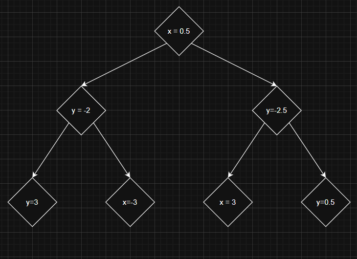
Here's what the root node does:

Here's what the second branch does:

Here's what the last branch does:

This would classify the points into different sections, each of them a different shade of red. This can be observed when we view this in top view. When we want to predict on a new point, all we need to do is put it through the root node and then let it trickle down the tree and see which section it lands into. Once we know the section, we take the average of the points in the section and predict that as the value.

Why is this method different?#

View top view to see how this is more of a multi-class classification problem than a regression problem.

Even though this is a regression problem, we split the data into feature space into different classes as seen above. Then if a point lies in a certain feature space, we average the values of the rest of the values in the training dataset and give the value as the prediction.

How to decide on the splits?#

Lets look at this from a very fundamental perspective. We want to split the data in a way such that the impurity reduces the most from the previous branch to this one. This is done using Variance Reduction. We calculate the Variance at the parent node. Then calculate the Variance at the daughter nodes. Let the Variance of parent nodes be $V_p$ , The variance of the daughter nodes $V_0$, $V_1$. And the ratio of division be $\omega_0$ and $\omega_1$. Ratio of division is the number of datapoints in that daughter node vs its parent node.

We want to reduce variance to the highest extent possible. This is done using an optimizer like SGD, Adam or so on. SGD and other optimizers usually change the parameters by reducing a certain function like MSE, MAE or other such loss functions. But here we want to increase the parameter Variance Reduction, so all we have to do is negate the value of Variance Reduction. Minimizing the value of Variance Reduction is the same as maximizing the negative of value of Variance reduction.

All that being said, we pick the split with maximum variance reduction at each split.